This entry is a cross post of the SMAC3 article. One of the core developers of SMAC3, Difan Deng, wrote the article below and Shuhei Watanabe from the Optuna team is posting this article on his behalf.
SMAC3 is developed by AutoML.org, mainly by the SMAC team, in Germany. AutoML.org is one of the world-leading AutoML research groups and the Optuna team collaborated with AutoML.org this time, having led to him a SMAC3-based sampler to OptunaHub. This article is about the newly introduced SMACSampler.
Introduction
SMAC3 [1] offers a robust and flexible framework for Bayesian Optimization to support users in determining well-performing hyperparameter configurations for their (machine learning) algorithms, datasets, and applications at hand. SMAC3 provides several default hyperparameter optimization pipelines for different use cases to make life easy. These default settings are summarized as Facades to provide users with a simple interface. However, users could also customize their optimization pipelines with SMAC3 components. For example, thanks to the modular design, researchers can easily benchmark different types of Bayesian optimization algorithms.
We introduced SMAC3 to OptunaHub this time and SMACSampler in OptunaHub also provides an interface for users to configure their Bayesian optimization pipeline, including but not limited to different types of initial designs, surrogate models, acquisition functions, and acquisition function optimizers. It is also possible to switch facades from the SMACSampler interface as well. In this article, we show some simple examples of SMACSampler.
To run the codes in this article, please install the dependencies as follows:
# Installation of Dependencies.
$ pip install optuna optunahub cmaes smac torch matplotlib
SMAC3 Registered on OptunaHub
SMACSampler in OptunaHub is, by default, based on HyperparameterOptimizationFacade, which uses Random Forest (RF) as a surrogate model and expects improvement (EI) with log transformation [2] as an acquisition function. To verify the efficiency of SMACSampler, we evaluate it on the Branin function. We optimize the difference between the evaluated Branin function value and the global minima, which we name regret. As a baseline, we used CMA-ES in Optuna. The result is shown in Figure 1. The horizontal axis shows the number of trials, and the vertical axis shows the regret (lower is better). The solid lines (blue: CMA-ES, orange: SMAC) show each optimizer’s minimum objective function value. As demonstrated, we can now easily compare samplers in Optuna with SMAC3.
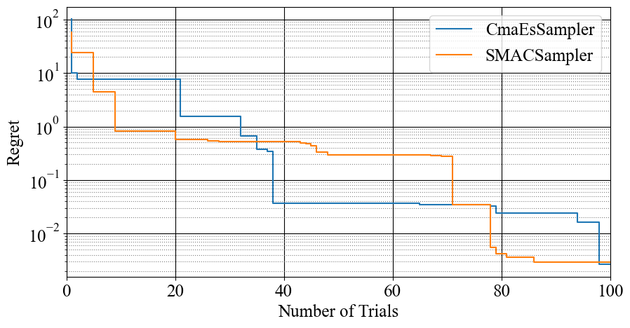
Figure 1. Comparison of SMAC (orange) and CMA-ES (blue) using Branin function.
The code used for benchmarking is as follows:
from __future__ import annotations

import matplotlib.pyplot as plt
import numpy as np
import optuna
from optuna.samplers import CmaEsSampler
import optunahub


n_trials = 100
SMACSampler = optunahub.load_module("samplers/smac_sampler").SMACSampler


def branin(x1: float, x2: float) -> float:
   # Branin function: https://www.sfu.ca/~ssurjano/branin.html
   a = 1
   b = 5.1 / (4*np.pi**2)
   c = 5 / np.pi
   r = 6
   s = 10
   t = 1 / (8 * np.pi)
   return a * (x2 - b * x1 ** 2 + c * x1 - r) ** 2 + s * (1-t) * np.cos(x1) + s


def objective(trial: optuna.Trial) -> float:
   x1 = trial.suggest_float("x1", -5.0, 10.0)
   x2 = trial.suggest_float("x2", 0.0, 15.0)
   # (-pi, 12.275) is one of the global minima for Branin function
   return branin(x1, x2) - branin(-np.pi, 12.275)


def plot_results(*samplers: optuna.samplers.BaseSampler) -> None:
   _, ax = plt.subplots(figsize=(10, 5))
   ax.set_yscale("log")
   for sampler in samplers:
       study = optuna.create_study(sampler=sampler)
       study.optimize(objective, n_trials=n_trials)
       values = np.minimum.accumulate([float(t.value) for t in study.get_trials()])
       ax.step(np.arange(n_trials) + 1, values, label=sampler.__class__.__name__)

   ax.set_xlim(0, n_trials)
   ax.set_xlabel("Number of Trials")
   ax.set_ylabel("Regret")
   ax.legend()
   ax.grid(which="minor", color="gray", linestyle=":")
   ax.grid(which="major", color="black")
   plt.show()


search_space = {
   "x1": optuna.distributions.FloatDistribution(-5., 10.),
   "x2": optuna.distributions.FloatDistribution(0., 15.),
}
seed = 42
plot_results(
   CmaEsSampler(seed=seed), SMACSampler(search_space, n_trials=n_trials, seed=seed)
)
Customize Your SMACSampler
Like SMAC3, users can customize their own SMACSampler in OptunaHub by passing the corresponding arguments. Currently, we allow users to customize:
- Surrogate model: gp for Gaussian process, gp_mcmc for Gaussian process with parameters sampled by MCMC, and rf for random forest,
- Acquisition function: ei for expected improvement, ei_log for expected improvement with log transformation [2], pi for the probability of improvement, and lcb for lower confidence bound
- Initialization design: sobol for the Sobol sequence, lhb for Latin hypercube, and random for uniform random.
We defer to SMAC3 | OptunaHub for further details.
Here is another example using SMACSampler, but with Gaussian process and expected improvement as the surrogate model and acquisition function. We compare this SMACSampler with Optuna GPSampler:
from optuna.samplers import GPSampler


plot_results(
   GPSampler(seed=seed),
   SMACSampler(search_space, surrogate_model_type="gp", acq_func_type="ei", n_trials=n_trials, seed=seed),
)
The result is shown in Figure 2:
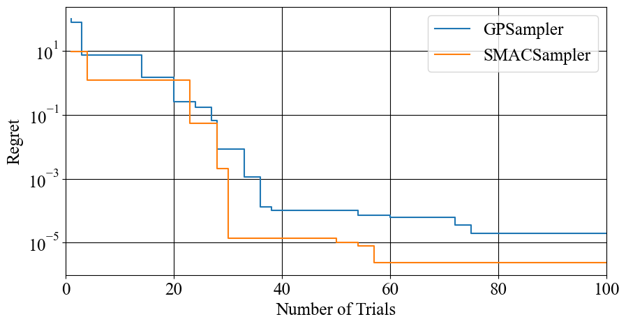
Figure 2. Comparison of SMAC GP (orange) and GP sampler (blue) using Branin function
Conclusion
This article introduced SMACSampler, a versatile Bayesian optimization for hyperparameter optimization, available on OptunaHub.
References
[1] Lindauer et al. “SMAC3: A Versatile Bayesian Optimization Package for Hyperparameter Optimization”, Journal of Machine Learning Research, http://jmlr.org/papers/v23/21-0888.html
[2] Watanabe, “Derivation of Closed Form of Expected Improvement for Gaussian Process Trained on Log-Transformed Objective”, arXiv preprint arXiv:2411.18095, https://arxiv.org/abs/2411.18095
Comments are closed